Ouster OS1 - first impressions
Recently I’ve started integrating Ouster OS1-16 on a client’s platform and he was nice enough to allow me to run some tests with this LiDAR sensor. This post describes my first impression with this unit and provides some pointers that can be useful for anyone looking into using Ouster sensors with Robot Operating System.
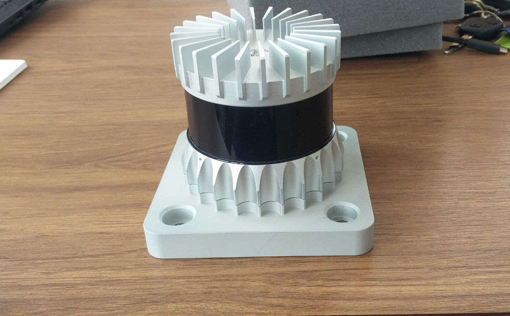
Hardware
| Parameter | Value |
|---|---|
| Range | 0.25-120m (at 80% reflectivity) |
| Range resolution | 0.3 cm |
| Horizontal FoV | 360° |
| Vertical FoV | 33.2° |
| Rotation frequency | 10 or 20Hz |
| Laser wavelength | 865nm |
| Operating power | 14-20W |
| Operating voltage | 24V |
| Interface | Gigabit Ethernet (UDP) |
| Price | ~3.5k USD |
Setup
Here are some useful links that should get you started if you wanted to use OS1 sensors:
- Ouster Resoures - Software User Guide is a must read before starting with this LiDAR
- Ouster ROS driver - The driver developed by the Ouster team
- ROS 2 Ouster Drivers - Drivers developed by Steve Macenski
- Building Maps Using Google Cartographer and the OS1 Lidar Sensor - Very useful tutorial
Networking
All the tutorials mention setting up DHCP for Ouster sensors, however, if you are able to find the sensor’s IP address then in my experience so far you can use it directly. For these initial tests, I’ve used IP only and didn’t have any issues with the Ouster Driver, Ouster studio, and connecting to the sensor using Netcat.
I found netcat to be very useful in my first tests the commands that I was running were:
nc 10.42.0.245 7501
get_sensor_info
get_time_info
set_config_param timestamp_mode TIME_FROM_PTP_1588
reinitialize
write_config_txt
Among these commands get_time_info was very useful to roughly check the sensor timestamp against my computer time and make sure the clocks are synchronized.
Time syncronization
Handling time properly is very important, especially if you want to display your data live in software like RVIZ. Here are the timing options that you can find in ouster (via the Software User Guide):
TIME_FROM_INTERNAL_OSC- Use the internal clock. Measurements are time stamped with ns since power-on. Free running counter based on the OS1’s internal oscillator. Counts seconds and nanoseconds since OS1 turn on, reported at ns resolution (both a second and nanosecond register in every UDP packet), but min increment is on the order of 10ns. Accuracy is +/- 90ppm.TIME_FROM_SYNC_PULSE_IN- A free running counter synced to the SYNC_PULSE_IN input counts seconds (#of pulses) and nanoseconds since OS1 turn on. If multipurpose_io_mode is set to INPUT_NMEA_UART then the seconds register jumps to time extracted from a NMEA$GPRMC message read on the multipurpose_io port. Reported at ns resolution (both a second and nanosecond register in every UDP packet), but min increment is on the order of 10 ns. Accuracy is +/- 1 s from a perfect SYNC_PULSE_IN source.TIME_FROM_PTP_1588- Synchronize with an external PTP master. A monotonically increasing counter that will begin counting seconds and nanoseconds since startup. As soon as a 1588 sync event happens, the time will be updated to seconds and nanoseconds since 1970. The counter must always count forward in time. If another 1588 sync event happens the counter will either jump forward to match the new time or slow itself down. It is reported at ns resolution (there is both a second and nanosecond register in every UDP packet), but the minimum increment varies. Accuracy is +/-<50us from the 1588 master.
Initially, I was trying to use TIME_FROM_SYNC_PULSE_IN with my ArduSimple boards. It worked OK but if you read the description of the mode above you’ll notice it says “If multipurpose_io_mode is set to INPUT_NMEA_UART then the seconds register jumps” - this explains why accuracy is +/- 1s from the pulse in source.
Another thing to note about using TIME_FROM_SYNC_PULSE_IN is that with 1.13 software there is a bug which causes the reported time to be off by 24 hours from the time provided.
If you need accurate timing then TIME_FROM_PTP_1588 is the way to go. Software User Guide has a very good workflow on how to set it up, even for a single machine. It’s best if machines support ethernet hardware timestamping but if it doesn’t the software timestamping seems to work well too.
Cartographer test
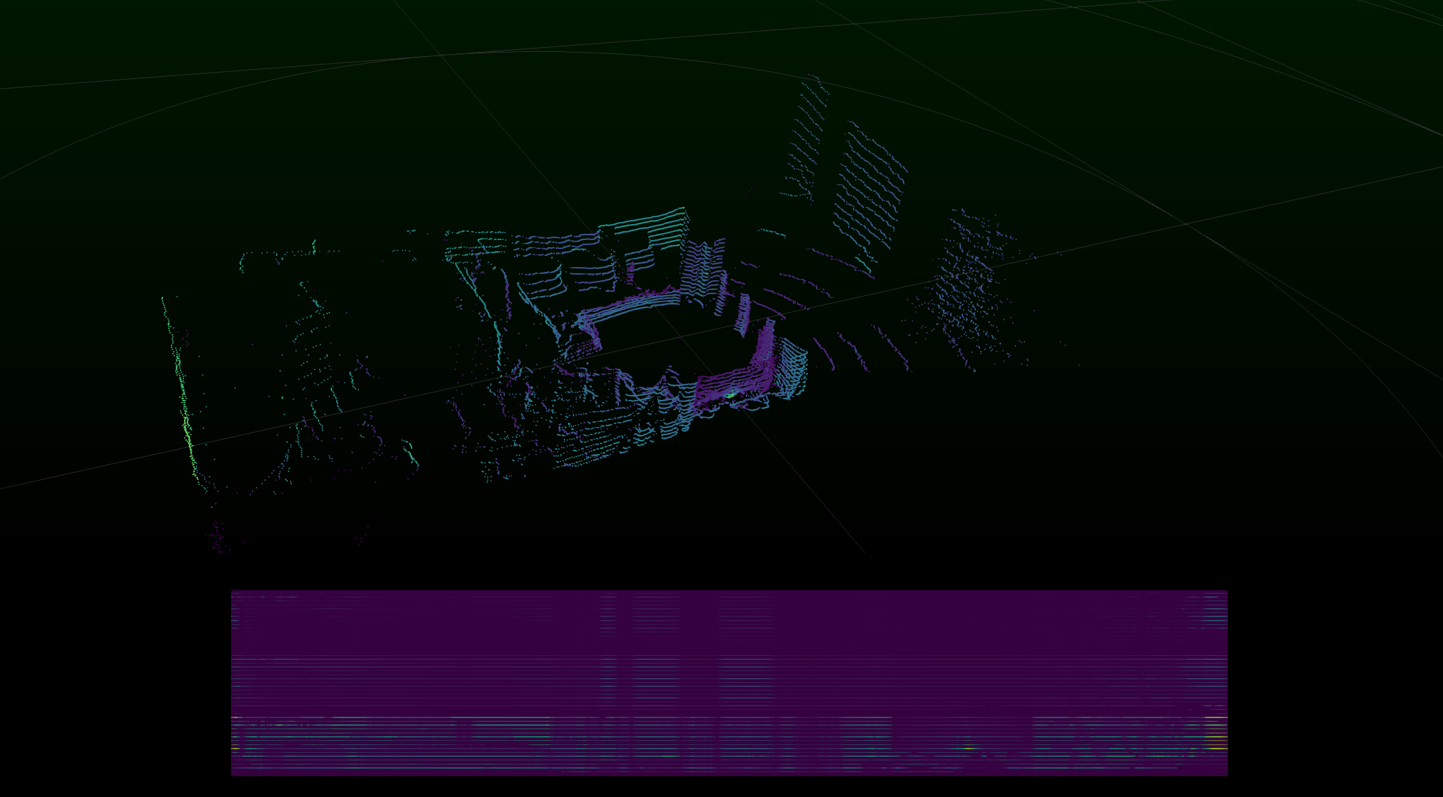
After making sure my launch files work with the sensor I’ve wanted to test some SLAM implementation. I ended up trying the sensor with Cartographer:
In my RVIZ settings, I’ve set the point cloud decay time to 4 seconds. As you can see the localization is not perfect but it’s not too bad, given I’ve used the default configuration from Ouster’s blog post on Cartographer integration.
Point cloud assembly
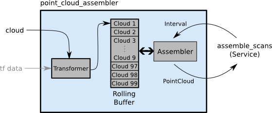
The second thing I wanted to discover for this blog post was the ways how to build a usable point cloud from the localized sensor data. This led me to point_cloud2_assembler from laser_assembler package. ROS Wiki describes this package as follows:
The laser_scan_assembler subscribes to sensor_msgs/LaserScan messages on the scan topic. These scans are processed by the Projector and Transformer, which project the scan into Cartesian space and then transform it into the fixed_frame. This results in a sensor_msgs/PointCloud that can be added to the rolling buffer. Clouds in the rolling buffer are then assembled on service calls.
To obtain this pointcloud I’ve added the following nodes to my launch file:
  <node type="point_cloud2_assembler" pkg="laser_assembler" name="my_assembler">
    <remap from="cloud" to="/os1_cloud_node/points"/>
    <param name="max_clouds" type="int" value="400" />
    <param name="fixed_frame" type="string" value="map" />
  </node>

  <node pkg="carto_demo" type="map_assembler.py" name="map_assembler"/>
where map_assembler.py is a simple Python script:
#!/usr/bin/env python

import rospy
from laser_assembler.srv import AssembleScans2
from sensor_msgs.msg import PointCloud2

rospy.init_node("map_assembler")
rospy.wait_for_service("assemble_scans2")
assemble_scans_srv = rospy.ServiceProxy('assemble_scans2', AssembleScans2)
pub = rospy.Publisher ("/assembled_pointcloud", PointCloud2, queue_size=1)

r = rospy.Rate(1)
last_time = rospy.Time(0,0)

while (not rospy.is_shutdown()):
    try:
        time_now = rospy.Time.now()
        resp = assemble_scans_srv(last_time, time_now)
        last_time = time_now
        pub.publish(resp.cloud)

    except rospy.ServiceException, e:
        print "Service call failed: %s"%e

    r.sleep()
Since I’ve ben saving all my data to a bag file I was then able to create an assembled pointcloud by running a bag_to_pcd node from pcl_ros with the following syntax:
rosrun pcl_ros bag_to_pcd <input_file.bag> <topic> <output_directory>
This command will create a .pcd file with the scan data that you can later import into software like CloudCompare:
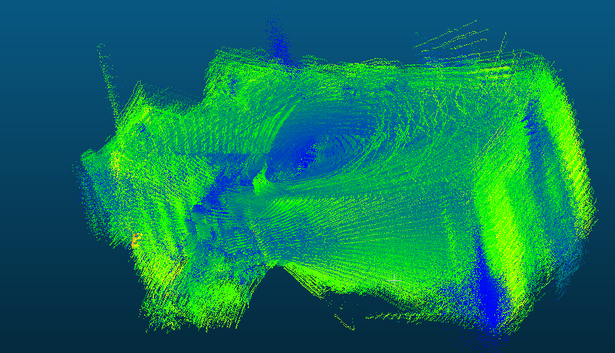
Looking at the point cloud you can notice quite many outliers. Most of them are most likely the result of me not tuning the Cartographer for this post, however, the single line of measurements in the top left side of the above image looks quite a bit odd. Since it happens to be where a window in my apartment is I’m wondering if this could be caused by light interference.
Next steps
I’ll be running further tests on this sensor as I’m working on the client’s project. If I come across any significant findings I’ll make sure to update this blog post. If you would still like to know more then you can find two videos about Ouster on Steve Macenski’s Robots For Robots YouTube Channel.